
Weighted regression
Weighted regression consists on assigning different weights to each observation and hence more or less importance at the time of fitting the regression.
On way to look at it is to think as solving the regression problem minimizing Weighted Mean Squared Error(WSME) instead of Mean Squared Error(MSE)
\[WMSE(\beta, w) = \frac{1}{N} \sum_{i=1}^n w_i(y_i - \overrightarrow {x_i} \beta)^2\] Intuitively, we are looking fot the coefficients that minimize MSE but putting different weights to each observation. OLS is a particular case where all the \(w_i = 1\)
Why doing this? A few reasons (Shalizi 2015. Chapter 7.1)
Focusing Accuracy: We want to predict specially well some particular points or region of points, maybe because that’s the focus for production or maybe because being wrong at those observations has a huge cost, etc. Using Weighted regression will do an extra effort to match that data.
Discount imprecision: OLS returns the maximum likelihood estimates when the residuals are independent, normal with mean 0 and with constant variance. When we face non constant variance OLS no longer returns the MLE. The logic behind using weighted regression is that makes no sense to pay equal attention to all the observations since some of them have higher variance and are less indicative of the conditional mean. We should put more emphasis on the regions of lower variance, predict it well and “expect to fit poorly where the noise is big”.
The weights that will return MLE are \(\frac{1}{\sigma_i^2}\)Sampling bias: If we think or know that the observations in our data are not completely random and some subset of the population might be under-represented (in a survey for example or because of data availability) it might make sense to weight observation inversely to the probability of being included in the sample. Under-represented observations will get more weights and over-represented less weight.
Another similar situation is related to covariate shift. If the distribution of variable x changes over time we can use a weight designed as the ratio of the probability density functions. > "If the old pdf was p(x) and the new one is q(x), the weight we’d want to is \(w_i=q(x_i)/p(x_i)\)Other: Related to GLM, when the conditional mean is a non linear function of a linear predictor. (Not further explained in the book at this point)
Is there a scenario where OLS is better than Weighted regression? Assuming we can compute the weights.
Example.
First we will see the impact of using weighted regression, using a simulated scenario where we actually know the variance of the error of each observation. This is not realistic but useful to see it in action.
library(tidyverse)We generate 1000 datapoints with a linear relation between y and x. Intercept = 0, slope = 5. We let the variance of the error depend on the value of x. Higher values of x are associated with higher values of the variance of the error.
set.seed(23)
n=1000
x = runif(n,0,10)
error = rnorm(n,0, x/1.5)
df = data.frame(x)
df = df %>% mutate(y = 5*x + error)
Visually..
ggplot(data=df, aes(x=x, y=y)) +
  geom_point(alpha=0.3) +
  # geom_smooth(color="blue") +
  # geom_smooth(method = "lm", mapping = aes(weight = (1/sqrt(x)^2)),
  #             color = "red", show.legend = FALSE) +
  NULL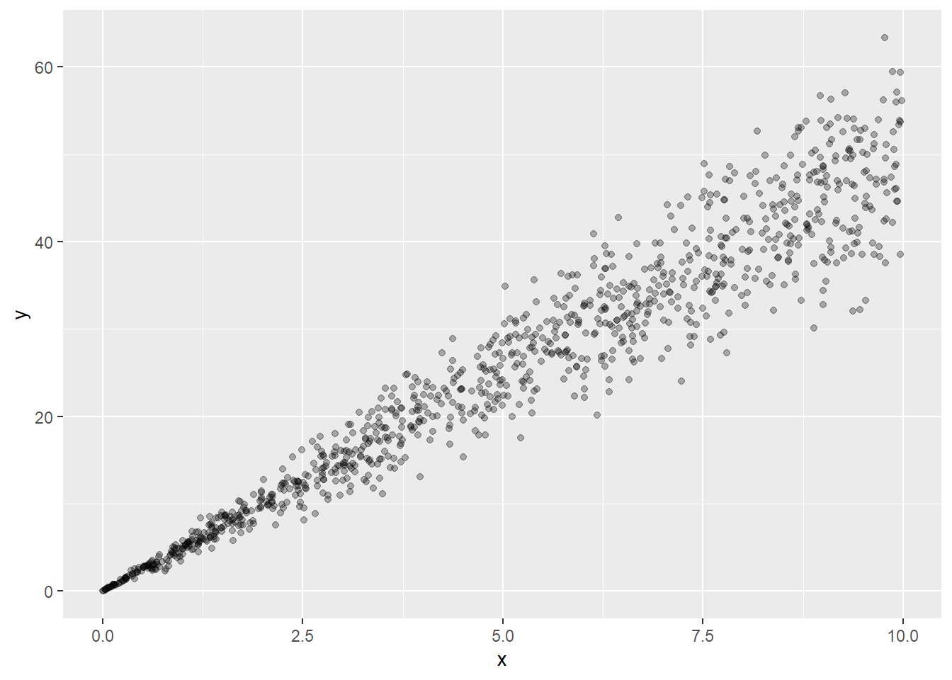
Linear regression
ols = lm(formula = "y~x", data=df)
summary(ols)
##
## Call:
## lm(formula = "y~x", data = df)
##
## Residuals:
## Min 1Q Median 3Q Max
## -14.868 -1.720 -0.137 1.918 14.722
##
## Coefficients:
## Estimate Std. Error t value Pr(>|t|)
## (Intercept) 0.19192 0.24278 0.791 0.429
## x 4.95585 0.04148 119.489 <2e-16 ***
## ---
## Signif. codes: 0 '***' 0.001 '**' 0.01 '*' 0.05 '.' 0.1 ' ' 1
##
## Residual standard error: 3.855 on 998 degrees of freedom
## Multiple R-squared: 0.9347, Adjusted R-squared: 0.9346
## F-statistic: 1.428e+04 on 1 and 998 DF, p-value: < 2.2e-16We get an intercept of 0.19, non-significant when the actual value is 0 and a slope of 4.96 when the actual value is 5.
Weighted linear regression
wols = lm(formula = "y~x", data=df, weights = (1/sqrt(x)^2) )
summary(wols)
##
## Call:
## lm(formula = "y~x", data = df, weights = (1/sqrt(x)^2))
##
## Weighted Residuals:
## Min 1Q Median 3Q Max
## -4.8880 -0.8601 -0.0016 0.8936 4.6535
##
## Coefficients:
## Estimate Std. Error t value Pr(>|t|)
## (Intercept) 0.001483 0.030072 0.049 0.961
## x 4.993473 0.021874 228.286 <2e-16 ***
## ---
## Signif. codes: 0 '***' 0.001 '**' 0.01 '*' 0.05 '.' 0.1 ' ' 1
##
## Residual standard error: 1.498 on 998 degrees of freedom
## Multiple R-squared: 0.9812, Adjusted R-squared: 0.9812
## F-statistic: 5.211e+04 on 1 and 998 DF, p-value: < 2.2e-16We get an intercept of 0, non-significant too but much closer to 0 and with lower standard error and a slope of 4.99 also much closer to the actual value of 5 and with lower standard error.
Conclusion: if we know the right weights we can get better estimates from a linear regression in case of heteroscedasticity.
